Create and run a simple CellML model: editing and simulation

In this example we create a simple CellML model and run it. The model is the Van der Pol oscillator[1] defined by the second order equation

\[\frac{d^{2}x}{dt^{2}} - \mu\left( 1 - x^{2} \right)\frac{\text{dx}}{\text{dt}} + x = 0\]

with initial conditions \(x = - 2;\ \frac{\text{dx}}{\text{dt}} = 0\). The parameter \(\mu\) controls the magnitude of the damping term. To create a CellML model we convert this to two first order equations[2] by defining the velocity \(\frac{\text{dx}}{\text{dt}}\) as a new variable \(y\):

(1)\[\frac{\text{dx}}{\text{dt}} =\ y\]

(2)\[\frac{\text{dy}}{\text{dt}} =\ \mu\left( 1 - x^{2} \right)y - x\]

The initial conditions are now \(x = - 2;y = 0\).

With the central pane in Editing mode (e.g. CellML Text view), create a new CellML file: File ‣ New ‣ CellML File and then type in the following lines of code after deleting the three lines that indicate where the code should go:

def model van_der_pol_model as
    def comp main as
        var t: dimensionless {init: 0};
        var x: dimensionless {init: -2};
        var y: dimensionless {init: 0};
        var mu: dimensionless {init: 1};
        // These are the ODEs
        ode(x,t)=y;
        ode(y,t)=mu*(1{dimensionless}-sqr(x))*y-x;
    enddef;
enddef;

Things to note[3] are:

1. the closing semicolon at the end of each line (apart from the first two def statements that are opening a CellML construct);

2. the need to indicate dimensions for each variable and constant (all dimensionless in this example – but more on dimensions later);

3. the use of ode(x,t) to indicate a first order[4] ODE in x and t

4. the use of the squaring function sqr(x) for \(x^{2}\), and

5. the use of ‘//’ to indicate a comment.

A partial list of mathematical functions available for OpenCOR is:

\(x^{2}\)	sqr(x)	\(\sqrt{x}\)	sqrt(x)	\(\ln x\)	ln(x)	\(\log_{10}x\)	log(x)	\(e^{x}\)	exp(x)	\(x^{a}\)	pow(x,a)
\(\sin x\)	sin(x)	\(\cos x\)	cos(x)	\(\tan x\)	tan(x)	\(\csc x\)	csc(x)	\(\sec x\)	sec(x)	\(\cot x\)	cot(x)
\(\sin^{-1}x\)	asin(x)	\(\cos^{-1} x\)	acos(x)	\(\tan^{-1} x\)	atan(x)	\(\csc^{-1} x\)	acsc(x)	\(\sec^{-1} x\)	asec(x)	\(\cot^{-1}x\)	acot(x)
\(\sinh x\)	sinh(x)	\(\cosh x\)	cosh(x)	\(\tanh x\)	tanh(x)	\(\operatorname{csch} x\)	csch(x)	\(\operatorname{sech} x\)	sech(x)	\(\coth x\)	coth(x)
\(\sinh^{-1} x\)	asinh(x)	\(\cosh^{-1} x\)	acosh(x)	\(\tanh^{-1} x\)	atanh(x)	\(\operatorname{csch}^{-1} x\)	acsch(x)	\(\operatorname{sech}^{-1}x\)	asech(x)	\(\coth^{-1} x\)	acoth(x)

Table 1. Partial list of mathematical functions available for coding in OpenCOR.

Positioning the cursor over either of the ODEs renders the maths in standard form above the code as shown in Fig. 3.

Note that CellML is a declarative language[5] (unlike say C, Fortran or Matlab, which are procedural languages) and therefore the order of statements does not affect the solution. For example, the order of the ODEs could equally well be

ode(y,t)=mu*(1{dimensionless}-sqr(x))*y-x;
ode(x,t)=y;

The significance of this will become apparent later when we import several CellML models to create a composite model.

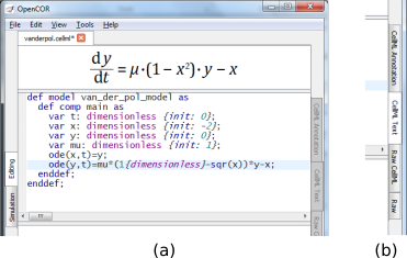
Fig. 3 (a) Positioning the cursor over an equation and clicking (shown by the highlighted line) renders the maths. (b) Once the model has been successfully saved, the CellML Text view tab becomes white rather than grey. The right hand tabs provide different views of the CellML code.

Now save the code to a local folder using Save under the File menu (File ‣ Save) (or ‘CTRL-S’) and choosing .cellml as the file format[6]. With the CellML model saved various views, accessed via the tabs on the right hand edge of the window, become available. One is the CellML Text view (the view used to enter the code above); another is the Raw CellML view that displays the way the model is stored and is intentionally verbose to ensure that the meaning is always unambiguous (note that positioning the cursor over part of the code shows the maths in this view also); and another is the Raw view. Notice that ‘CTRL-T’ in the Raw CellML view performs validation tests on the CellML model. The CellML Text view provides a much more convenient format for entering and editing the CellML model.

With the equations and initial conditions defined, we are ready to run the model. To do this, click on the Simulation tab on the left hand edge of the window. You will see three main areas - at the left hand side of the window are the Simulation, Solvers, Graphs and Parameters panels, which are explained below. At the right hand side is the graphical output window, and running along the bottom of the window is a status area, where status messages are displayed.

Simulation Panel

This area is used to set up the simulation settings.

• Starting point - the value of the variable of integration (often time) at which the simulation will begin. Leave this at 0.

• Ending point - the point at which the simulation will end. Set to 100.

• Point interval - the interval between data points on the variable of integration. Set to 0.1.

Just above the Simulation panel are controls for running the simulation. These are:

Run (), Pause (), Reset parameters (), Clear simulation data (), Interval delay (), Add()/Subtract() graphical output windows and Output solution to a CSV file ().

For this model, we suggest that you create three graphical output windows using the + button.

Solvers Panel

This area is used to configure the solver that will run the simulation.

• Name - this is used to set the solver algorithm. It will be set by default to be the most appropriate solver for the equations you are solving. OpenCOR allows you to change this to another solver appropriate to the type of equations you are solving if you choose to. For example, CVODE for ODE (ordinary differential equation) problems, IDA for DAE (differential algebraic equation) problems, KINSOL for NLA (non-linear algebraic) problems[7].

• Other parameters for the chosen solver – e.g. Maximum step, Maximum number of steps, and Tolerance settings for CVODE and IDA. For more information on the solver parameters, please refer to the documentation for the particular solver.

Note: these can all be left at their default values for our simple demo problem[8].

Graphs Panel

This shows what parameters are being plotted once these have been defined in the Parameters panel. These can be selected/deselected by clicking in the box next to a parameter.

Parameters Panel

This panel lists all the model parameters, and allows you to select one or more to plot against the variable of integration or another parameter in the graphical output windows. OpenCOR supports graphing of any parameter against any other. All variables from the model are listed here, arranged by the components in which they appear, and in alphabetical order. Parameters are displayed with their variable name, their value, and their units. The icons alongside them have the following meanings:

Editable constant	Editable state variable
Computed constant	Rate variable
Variable of integration	Algebraic quantity

Right clicking on a parameter provides the options for displaying that parameter in the currently selected graphical output window. With the cursor highlighting the top graphical output window (a blue line appears next to it), select x then Plot Against Variable of Integration – in this case t - in order to plot x(t). Now move the cursor to the second graphical output window and select y then t to plot y(t). Finally select the bottom graphical output window, select y and select Plot Against then Main then x to plot y(x).

Now click on the Run control. You will see a progress bar running along the bottom of the status window. Status messages about the successful simulation, including the time taken, are displayed in the bottom panel. This can be hidden by dragging down on the bar just above the panel. Fig. 4 shows the results. Use the interval delay wheel to slow down the plotting if you want to watch the solution evolve. You can also pause the simulation at any time by clicking on the Run control and if you change a parameter during the pause, the simulation will continue (when you click the Run control button again) with the new parameter.

Note that the values shown for the various parameters are the values they have at the end of the solution run. To restore these to their initial values, use the Reset parameters () button. To clear the graphical output traces, click on the Clear simulation data () button.

The top two graphical output panels are showing the time-dependent solution of the x and y variables. The bottom panel shows how y varies as a function of x. This is called the solution in state space and it is often useful to analyse the state space solution to capture the key characteristics of the equations being solved.

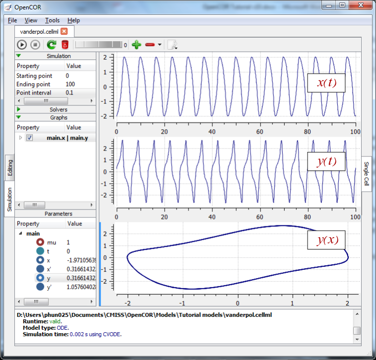
Fig. 4 Graphical output from OpenCOR. The top window is x(t), the middle is y(t) and the bottom is y(x). The Graphs panel shows that y(x) is being plotted on the graph output window highlighted by the LH blue line. The window at the very bottom provides runtime information on the type of equation being solved and the simulation time (2ms in this case). The computed variables shown in the left hand panel are at the values they have at the end of the simulation.

To obtain numerical values for all variables (i.e. x(t) and y(t)), click on the CSV file button (). You will be asked to enter a filename and type (use .csv). Opening this file (e.g. with Microsoft Excel) provides access to the numerical values. Other output types (e.g. BiosignalML) will be available in future versions of OpenCOR.

You can move the graphical output traces around with ‘left click and drag’ and you can change the horizontal or vertical scale with ‘right click and drag’. Holding the SHIFT key down while clicking on a graphical output panel allows you to interrogate the solution at any point. Right clicking on a panel provides zoom facilities.

Note

The simulation described above can also be loaded and run directly in OpenCOR using this link.

The various plugins used by OpenCOR can be viewed under the Tools menu. A French language version of OpenCOR is also available under the Tools menu. An option under the File menu allows a file to be locked (also ‘CTRL-L’). To indicate that the file is locked, the background colour switches to pink in the CellML Text and Raw CellML views and a lock symbol appears on the filename tab. Note that OpenCOR text is case sensitive.

---

Footnotes

[1]

http://en.wikipedia.org/wiki/Van_der_Pol_oscillator

[2]

Equations (1) and (2) are equations that are implemented directly in OpenCOR.

[3]

For more on the CellML Text view see http://opencor.ws/user/plugins/editing/CellMLTextView.html.

[4]

Note that a more elaborated version of this is ode(x, t, 1{dimensionless}) and a 2^nd order ODE can be specified as ode(x, t, 2{dimensionless}). 1^st order is assumed as the default.

[5]

Note also that the mathematical expressions in CellML are based on MathML – see http://www.w3.org/Math/

[6]

Note that .cellml is not strictly required but is best practice.

[7]

Other solvers include forward Euler, Heun and Runga-Kutta solvers (RK2 and RK4).

[8]

Note that a model that requires a stimulus protocol should have the maximum step value of the CVODE solver set to the length of the stimulus.