The Lorenz attractor
An example of a third order ODE system (i.e. three 1st order equations) is the Lorenz equations[1].
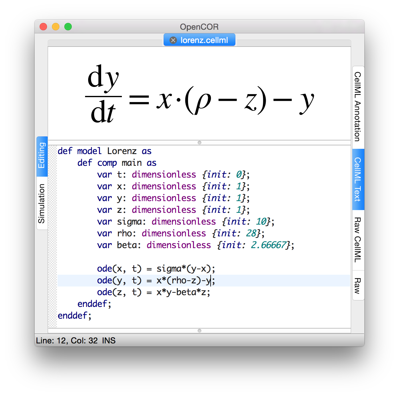
Fig. 9 CellML Text code for the Lorenz equations.
This system has three equations:
where \(\sigma,\ \rho\) and \(\beta\) are parameters.
The CellML Text code entered for these equations is shown in Fig. 9 with parameters
\(\sigma = 10\), \(\rho = 28\), \(\beta = 8/3\) = 2.66667
and initial conditions
\(x\left( 0 \right) = y\left( 0 \right) = z\left( 0 \right) =\)1.
Solutions for \(x\left( t \right)\), \(y\left( x \right)\) and \(z\left( x \right)\), corresponding to the time integration parameters shown on the LHS, are shown in Fig. 10. Note that this system exhibits ‘chaotic dynamics’ with small changes in the initial conditions leading to quite different solution paths.
This example illustrates the value of OpenCOR’s ability to plot variables as they are computed. Use the Simulation Delay wheel to slow down the plotting by a factor of about 5-10,000 - in order to follow the solution as it spirals in ever widening trajectories around the left hand wing of the attractor before coming close to the origin that then sends it off to the right hand wing of the attractor.
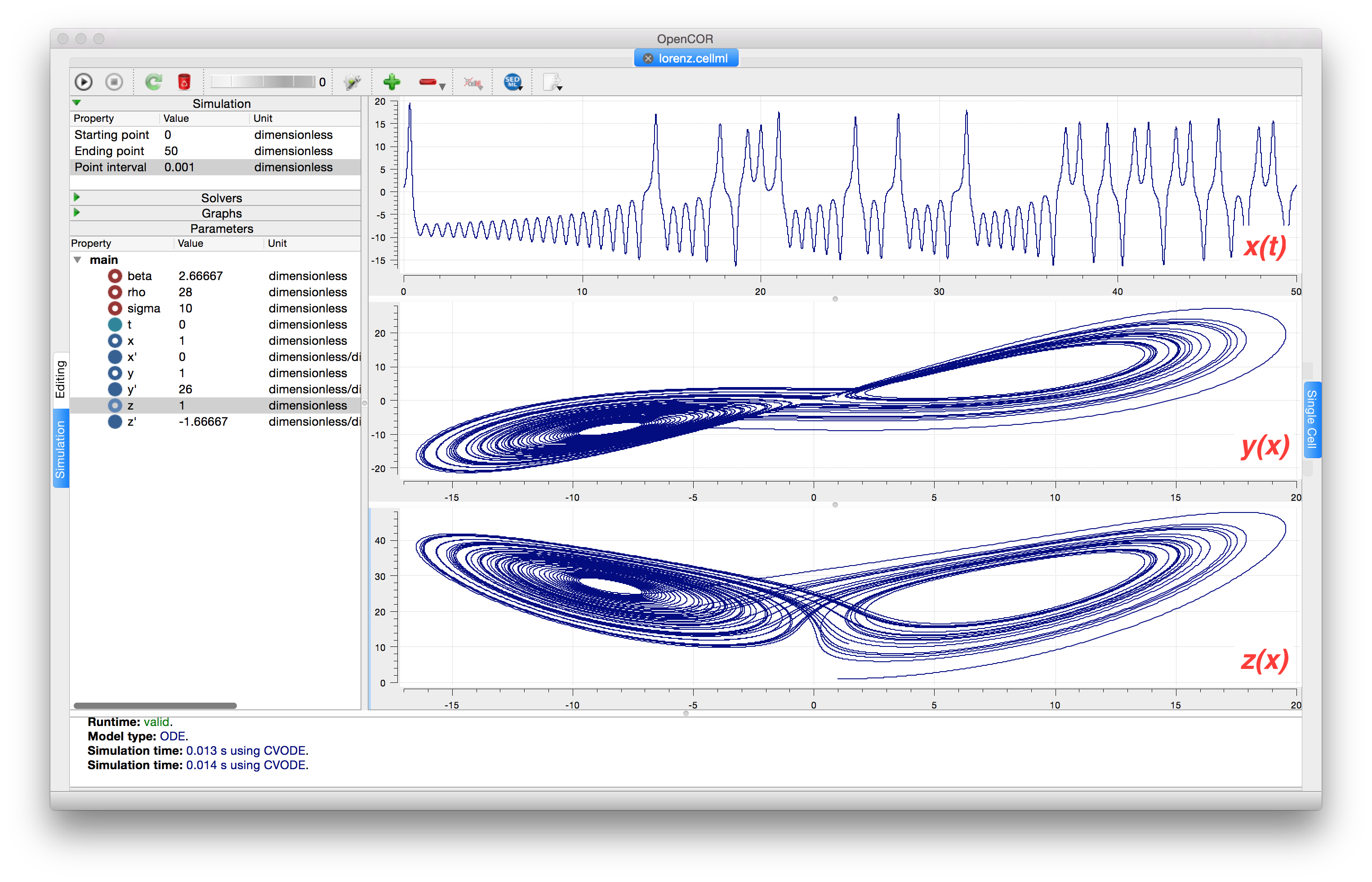
Fig. 10 Solutions of the Lorenz equations. Note that the parameters on the left have been reset to their initial values for this figure – normally they would be at their final solution values.
Solutions to the Lorenz equations are organised by the 2D ‘Lorenz manifold’. This surface has a very beautiful shape and has become an art form - even rendered in crochet![2] (See Fig. 11).
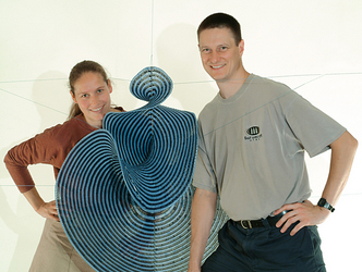
Fig. 11 The crocheted Lorenz manifold made by Professors Hinke Osinga and Bernd Krauskopf of the Mathematics Department at the University of Auckland, New Zealand.
Exercise for the reader
Another example of intriguing and unpredictable behaviour from a simple deterministic ODE system is the ‘blue sky catastrophe’ model [JH02] defined by the following equations:
with parameter \(A = 0.2645\) and initial conditions \(x\left( 0 \right) = 0.9\), \(y\left( 0 \right) = 0.4\). Run to \(t = 500\) with \(\Delta t = 0.01\) and plot \(x\left( t \right)\) and \(y\left( x \right)\) (OpenCOR link). Also try with \(A = 0.265\) to see how sensitive the solution is to small changes in parameter values.
Footnotes