A model of the potassium channel: Introducing CellML components and connections
We now deal specifically with the application of the previous model to the Hodgkin and Huxley (HH) potassium channel. Following the convention introduced by Hodgkin and Huxley, the gating variable for the potassium channel is \(n\) and the number of gates in series is \(\gamma = 4\), therefore
\(i_{K} = \bar{i_K}n^{4} = n^{4}\bar{g}_{K}\left( V - E_{K} \right)\)
where \(\bar{g}_{K} = \ 36 \text{mS.cm}^{-2}\), and with intra- and extra-cellular concentrations \(\left\lbrack K^{+} \right\rbrack_{i} = 90\text{mM}\) and \(\left\lbrack K^{+} \right\rbrack_{o} = 3\text{mM}\), respectively, the Nernst potential for the potassium channel (\(z = 1\) since one +ve charge on \(K^{+}\)) is
\(E_{k} = \frac{\text{RT}}{\text{zF}}\ ln\frac{\left\lbrack K^{+} \right\rbrack_{o}}{\left\lbrack K^{+} \right\rbrack_{i}} = 25\ ln\frac{3}{90} = - 85\text{mV}\).
As noted above, this is called the equilibrium potential since it is the potential across the cell membrane when the channel is open but no current is flowing because the electrostatic driving force from the potential (voltage) difference between internal and external ion charges is exactly matched by the entropic driving force from the ion concentration difference. \(n^{4}\bar{g}_{K}\) is the channel conductance.
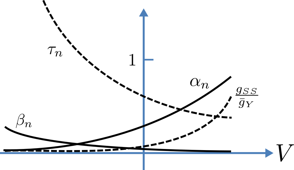
Fig. 18 Voltage dependence of rate constants \(\alpha_n\) and \(\beta_n\ (\text{ms}^{-1})\), time constant \(\tau_n\ (\text{ms})\) and relative conductance \(\frac{g_{SS}}{\bar{g}_Y}\).
The gating kinetics are described (as before) by
\(\frac{\text{dn}}{\text{dt}} = \alpha_{n}\left( 1 - n \right) - \beta_{n}\text{.n}\)
with time constant \(\tau_{n} = \frac{1}{\alpha_{n} + \beta_{n}}\) (see A simple first order ODE).
The main difference from the gating model in our previous example is that Hodgkin and Huxley found it necessary to make the rate constants functions of the membrane potential \(V\) (see Fig. 18) as follows[1]:
\(\alpha_{n} = \frac{- 0.01\left( V + 65 \right)}{e^{\frac{- \left( V + 65 \right)}{10}} - 1}\); \(\beta_{n} = 0.125e^{\frac{- \left( V + 75 \right)}{80}}\) .
Note that under steady state conditions when \(t \rightarrow \infty\) and
\(\frac{\text{dn}}{\text{dt}} \rightarrow 0\), \(\left. \ n \right|_{t = \infty} = n_{\infty} = \frac{\alpha_{n}}{\alpha_{n} + \beta_{n}}\).
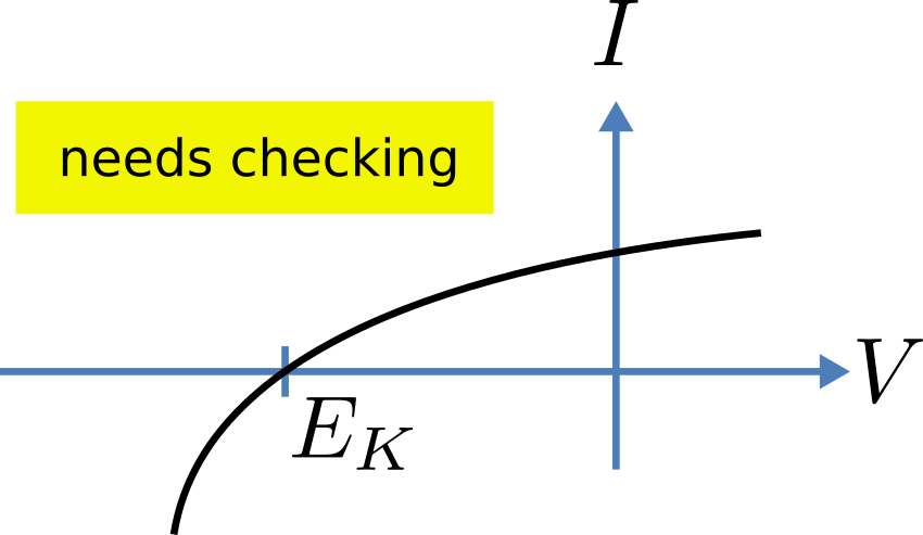
Fig. 19 The steady-state current-voltage relation for the potassium channel.
The voltage dependence of the steady state channel conductance is then
\(g_{\text{SS}} = \left( \frac{\alpha_{n}}{\alpha_{n} + \beta_{n}} \right)^{4}.\bar{g}_{Y}\).
(see Fig. 18). The steady state current-voltage relation for the channel is illustrated in Fig. 19.
These equations are captured with OpenCOR CellML Text view (together with the previous unit definitions) below. But first we need to explain some further CellML concepts.
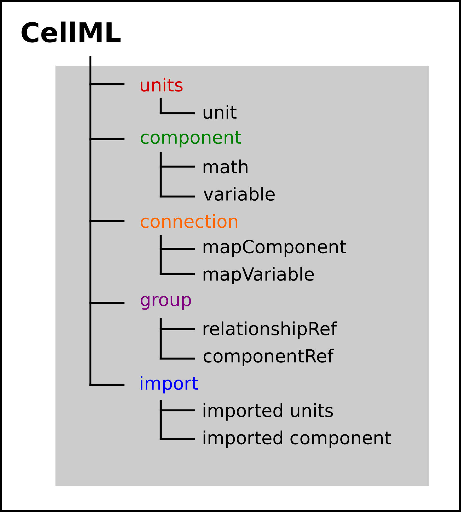
Fig. 20 Key entities in a CellML model.
We introduced CellML units above. We now need to introduce three more CellML constructs: components, connections (mappings between components) and groups. For completeness we also show one other construct in Fig. 20, imports, that will be used later in A model of the nerve action potential: Introducing CellML imports.
Defining components serves two purposes: it preserves a modular structure for CellML models, and allows these component modules to be imported into other models, as we will illustrate later [DPPJ03]. For the potassium channel model we define components representing (i) the environment, (ii) the potassium channel conductivity, and (iii) the dynamics of the n-gate.
Since certain variables (t, V and n) are shared between components, we need to also define the component maps as indicated in the CellML Text view below.
The CellML Text code for the potassium ion channel model is as follows[2]:
 1def model potassium_ion_channel as
 2   def unit millisec as
 3      unit second {pref: milli};
 4   enddef;
 5   def unit per_millisec as
 6      unit second {pref: milli, expo: -1};
 7   enddef;
 8   def unit millivolt as
 9      unit volt {pref: milli};
10   enddef;
11   def unit per_millivolt as
12      unit millivolt {expo: -1};
13   enddef;
14   def unit per_millivolt_millisec as
15      unit per_millivolt;
16      unit per_millisec;
17   enddef;
18   def unit microA_per_cm2 as
19      unit ampere {pref: micro};
20      unit metre {pref: centi, expo: -2};
21   enddef;
22   def unit milliS_per_cm2 as
23      unit siemens {pref: milli};
24      unit metre {pref: centi, expo: -2};
25   enddef;
26   def unit mM as
27      unit mole {pref: milli};
28   enddef;
29   def comp environment as
30      var V: millivolt { pub: out};
31      var t: millisec {pub: out};
32      V = sel
33      case (t > 5 {millisec}) and (t < 15 {millisec}):
34         -85.0 {millivolt};
35      otherwise:
36         0.0 {millivolt};
37      endsel;
38   enddef;
39   def group as encapsulation for
40      comp potassium_channel incl
41         comp potassium_channel_n_gate;
42      endcomp;
43   enddef;
44   def comp potassium_channel as
45      var V: millivolt {pub: in , priv: out};
46      var t: millisec {pub: in, priv: out};
47      var n: dimensionless {priv: in};
48      var i_K: microA_per_cm2 {pub: out};
49      var g_K: milliS_per_cm2 {init: 36};
50      var Ko: mM {init: 3};
51      var Ki: mM {init: 90};
52      var RTF: millivolt {init: 25};
53      var E_K: millivolt;
54      var K_conductance: milliS_per_cm2 {pub: out};
55      E_K=RTF*ln(Ko/Ki);
56      K_conductance = g_K*pow(n, 4{dimensionless});
57      i_K = K_conductance*(V-E_K);
58   enddef;
59   def comp potassium_channel_n_gate as
60      var V: millivolt {pub: in};
61      var t: millisec {pub: in};
62      var n: dimensionless {init: 0.325, pub: out};
63      var alpha_n: per_millisec;
64      var beta_n: per_millisec;
65      alpha_n = 0.01{per_millivolt_millisec}*(V+10{millivolt})
66         /(exp((V+10{millivolt})/10{millivolt})-1{dimensionless});
67      beta_n = 0.125{per_millisec}*exp(V/80{millivolt});
68      ode(n, t) = alpha_n*(1{dimensionless}-n)-beta_n*n;
69   enddef;
70   def map between environment and potassium_channel for
71      vars V and V;
72      vars t and t;
73   enddef;
74   def map between potassium_channel and
75     potassium_channel_n_gate for
76      vars V and V;
77      vars t and t;
78      vars n and n;
79   enddef;
80enddef;
Note that several other features have been added:
the event control select case which indicates that the voltage is specified to jump from 0 mV to -85 mV at t = 5 ms then back to 0 mV at t = 15 ms. This is only used here in order to test the K channel model; when the potassium_channel component is later imported into a neuron model, the environment component is not imported.
the use of encapsulation to embed the potassium_channel_n_gate inside the potassium_channel. This avoids the need to establish mappings from environment to potassium_channel_n_gate since the gate component is entirely within the channel component.
the use of \(\left\{ pub:in \right\}\) and \(\left\{ pub:out \right\}\) to indicate which variables are either supplied as inputs to a component or produced as outputs from a component[3]. Any variables not labelled as in or out are local variables or parameters defined and used only within that component. Public (and private) interfaces are discussed in more detail in the next section.
We now use OpenCOR, with Ending point 40 and Point interval 0.1, to solve the equations for the potassium channel under a voltage step condition in which the membrane voltage is clamped initially at 0mV and then stepped down to -85mV for 10ms before being returned to 0mV. At 0mV, the steady state value of the n gate is \(n_{\infty} = \frac{\alpha_{n}}{\alpha_{n} + \beta_{n}} =\) 0.324 and, at -85mV, \(n_{\infty} = \ \)0.945.
The voltage traces are shown at the top of Figure 21. The n-gate response, shown next, is to open further from its partially open value of \(n =\)0.324 at 0mV and then plateau at an almost fully open state of \(n =\)0.945 at the Nernst potential -85mV before closing again as the voltage is stepped back to 0mV. Note that the gate opening behaviour (set by the voltage dependence of the \(\alpha_{n}\) opening rate constant) is faster than the closing behaviour (set by the voltage dependence of the \(\beta_{n}\) closing rate constant). The channel conductance (\(= n^{4}\bar{g}_K\)) is shown next – note the initial s-shaped conductance increase caused by the \(n^{4}\) (four gates in series) effect on conductance. Finally the channel current \(i_{K} =\) conductance x \(\left( V - E_{K} \right)\) is shown at the bottom. Because the voltage is clamped at the Nernst potential (-85mV) during the period when the gate is opening, there is no current flow, but when the voltage is stepped back to 0mV, the open gates begin to close and the conductance declines but now there is a voltage gradient to drive an outward (positive) current flow through the partially open channel – albeit brief since the channel is closing.
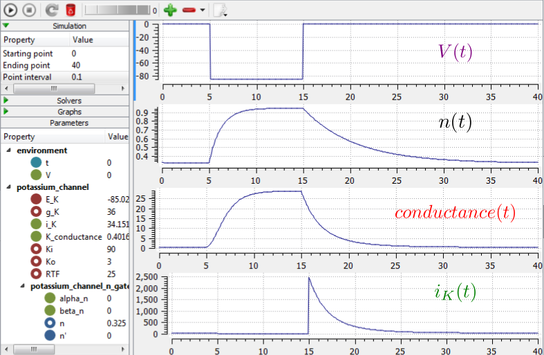
Fig. 21 Kinetics of the potassium channel gates for a voltage step from 0mV to -85mV (OpenCOR link). The voltage clamp step is shown at the top, then the n gate first order response, then the channel conductance, then the channel current. Notice how the conductance is slightly slower to turn on (due to the four gates in series) but fast to inactivate. Current only flows when there is a non-zero conductance and a non-zero voltage gradient. This is called the ‘tail current’.
Note that the CellML Text code above includes the Nernst equation with its dependence on the concentrations \(\left\lbrack K^{+} \right\rbrack_{i}\)= 90mM and \(\left\lbrack K^{+} \right\rbrack_{o}\)= 3mM. Try raising the external potassium concentration to \(\left\lbrack K^{+} \right\rbrack_{o}\)= 10mM – you will then see the Nernst potential increase from -85mV to -55mV and a negative (inward) current flowing during the period when the membrane voltage is clamped to -85mV. The cell is now in a ‘hyperpolarised’ state because the potential is less than the equilibrium potential.
Note that you can change a model parameter such as \(\left\lbrack K^{+} \right\rbrack_{o}\) either by changing the value in the left hand Parameters window (which leaves the file unchanged) or by editing the CellML Text code (which does change the file when you save from CellML Text view – which you have to do to see the effect of that change.
This potassium channel model will be used later, along with a sodium channel model and a leakage channel model, to form the Hodgkin-Huxley neuron model, where the membrane ion channel current flows are coupled to the equations governing current flow along the axon to generate an action potential.
Footnotes