A model of the nerve action potential: Introducing CellML imports
Here we describe the first (and most famous) model of nerve fibre electrophysiology based on the membrane ion channels that we have discussed in the last two sections. This is the work by Alan Hodgkin and Andrew Huxley in 1952 [AAF52] that won them (together with John Eccles) the 1963 Noble prize in Physiology or Medicine for “their discoveries concerning the ionic mechanisms involved in excitation and inhibition in the peripheral and central portions of the nerve cell membrane”.
Cable equation
The cable equation was developed in 1890[1] to predict the degradation of an electrical signal passing along the transatlantic cable. It is derived as follows:
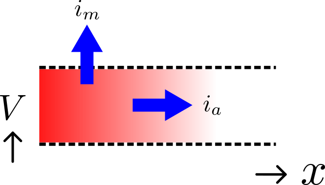
Fig. 24 Current flow in a leaky cable.
If the voltage is raised at the left hand end of the cable (shown by the deep red in Fig. 24), a current \(i_{a}\) (A) will flow that depends on the voltage gradient, given by \(\frac{\partial V}{\partial x}\) (\(V.m^{-1}\)) and the resistance \(r_{a}\) (\(\Omega.m^{-1}\)), Ohm’s law gives \(- \frac{\partial V}{\partial x} = r_{a}i_{a}\) . But if the cable leaks current \(i_{m}\) (\(A.m^{-1}\)) per unit length of cable, conservation of current gives \(\frac{\partial i_{a}}{\partial x} = i_{m}\) and therefore, substituting for \(i_{a}\) , \(\frac{\partial}{\partial x}\left( - \frac{1}{r_{a}}\frac{\partial V}{\partial x} \right) = i_{m}\) . There are two sources of membrane current \(i_{m}\) , one associated with the capacitance \(C_{m}\) (\(\approx 1\mu F/\text{cm}^{2}\)) of the membrane, \(C_{m}\frac{\partial V}{\partial t}\), and one associated with holes or channels in the membrane, \(i_{\text{leak}}\). Inserting these into the RHS gives
Rearranging gives the cable equation (for constant \(r_{a}\)):
where all terms represent current density (current per membrane area) and have units of \(\mu A/\text{cm}^{2}\).
Action potentials
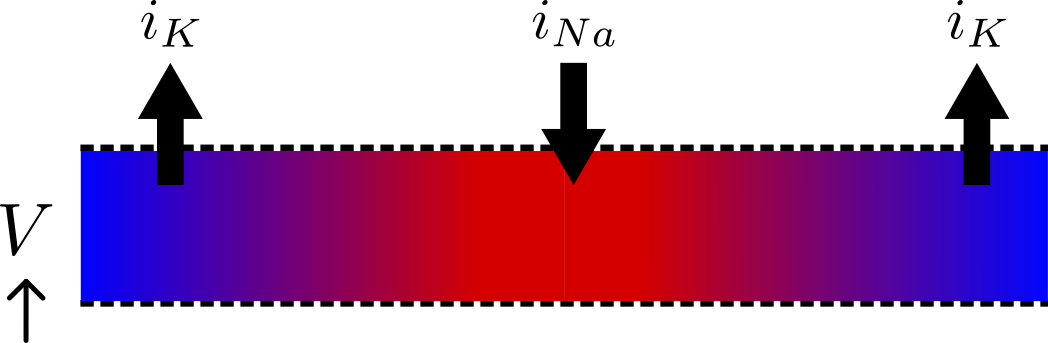
Fig. 25 Current flow in a neuron.
The cable equation can be used to model the propagation of an action potential along a neuron or any other excitable cell. The ‘leak’ current is associated primarily with the inward movement of sodium ions through the membrane ‘sodium channel’, giving the inward membrane current \(i_{\text{Na}}\), and the outward movement of potassium ions through a membrane ‘potassium channel’, giving the outward current \(i_{K}\) (see Fig. 25). A further small leak current \(i_{L} = g_{L}\left( V - E_{L} \right)\) associated with chloride and other ions is also included.
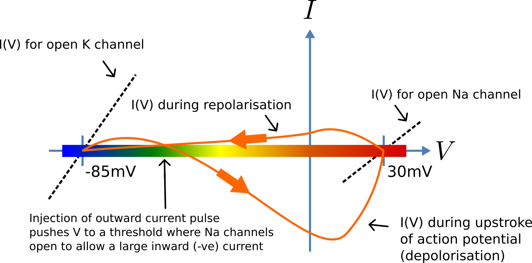
Fig. 26 Current-voltage trajectory during an action potential.
When the membrane potential \(V\) rises due to axial current flow, the Na channels open and the K channels close, such that the membrane potential moves towards the Nernst potential for sodium. The subsequent decline of the Na channel conductance and the increasing K channel conductance as the voltage drops rapidly repolarises the membrane to its resting potential of -85mV (see Fig. 26).
We can neglect[2] the term (\(- \frac{1}{r_{a}}\frac{\partial^{2}V}{\partial x^{2}}\)) (the rate of change of axial current along the cable) for the present models since we assume the whole cell is clamped with an axially uniform potential. We can therefore obtain the membrane potential \(V\) by integrating the first order ODE
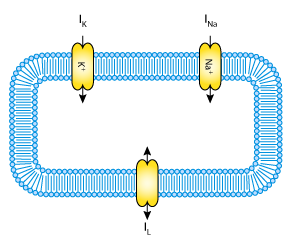
Fig. 27 A schematic cell diagram describing the current flows across the cell bilipid membrane that are captured in the Hodgkin-Huxley model. The membrane ion channels are a sodium (Na+) channel, a potassium (K+) channel, and a leakage (L) channel (for chloride and other ions) through which the currents INa, IK and IL flow, respectively.
We use this example to demonstrate the importing feature of CellML. CellML imports are used to bring a previously defined CellML model of a component into the new model (in this case the Na and K channel components defined in the previous two sections, together with a leakage ion channel model specified below). Note that importing a component brings the children components with it along with their connections and units, but it does not bring the siblings of that component with it.
To establish a CellML model of the HH equations we first lay out the model components with their public and private interfaces (Fig. 28).
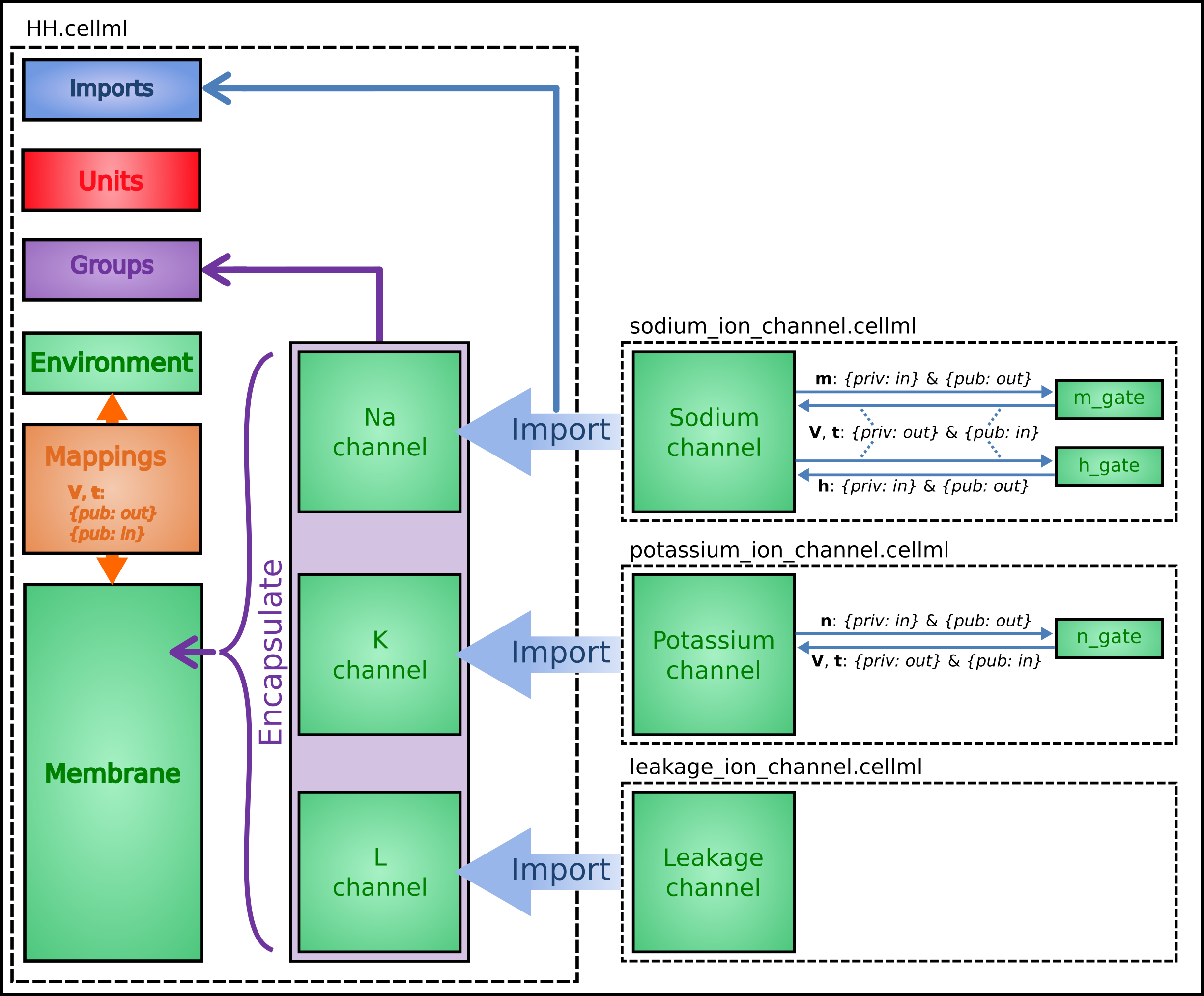
Fig. 28 Overall structure of the HH CellML model showing the encapsulation hierarchy (purple), the CellML model imports (blue) and the other key parts (units, components, and mappings) of the top level CellML model.
The HH model is the top level model. The CellML Text code for the HH model, together with the leakage_channel model, is given below. The imported potassium_ion_channel model and sodium_ion_channel model are unchanged from the previous sections
def model HH as
   def import using "sodium_ion_channel.cellml" for
      comp Na_channel using comp sodium_channel;
   enddef;
   def import using "potassium_ion_channel.cellml" for
      comp K_channel using comp potassium_channel;
   enddef;
   def import using "leakage_ion_channel.cellml" for
      comp L_channel using comp leakage_channel;
   enddef;
   def unit millisec as
      unit second {pref: milli};
   enddef;
   def unit millivolt as
      unit volt {pref: milli};
   enddef;
   def unit microA_per_cm2 as
      unit ampere {pref: micro};
      unit metre {pref: centi, expo: -2};
   enddef;
   def unit microF_per_cm2 as
      unit farad {pref: micro};
      unit metre {pref: centi, expo: -2};
   enddef;
   def group as encapsulation for
      comp membrane incl
         comp Na_channel;
         comp K_channel;
         comp L_channel;
      endcomp;
   enddef;
   def comp environment as
      var V: millivolt {init: -85, pub: out};
      var t: millisec {pub: out};
   enddef;
   def map between environment and membrane for
      vars V and V;
      vars t and t;
   enddef;
   def map between membrane and Na_channel for
      vars V and V;
      vars t and t;
      vars i_Na and i_Na;
   enddef;
   def map between membrane and K_channel for
      vars V and V;
      vars t and t;
      vars i_K and i_K;
   enddef;
   def map between membrane and L_channel for
      vars V and V;
      vars i_L and i_L;
   enddef;
   def comp membrane as
      var V: millivolt {pub: in, priv: out};
      var t: millisec {pub: in, priv: out};
      var i_Na: microA_per_cm2 {pub: out, priv: in};
      var i_K: microA_per_cm2 {pub: out, priv: in};
      var i_L: microA_per_cm2 {pub: out, priv: in};
      var Cm: microF_per_cm2 {init: 1};
      var i_Stim: microA_per_cm2;
      var i_Tot: microA_per_cm2;
      i_Stim = sel
      case (t >= 1{millisec}) and (t <= 1.2{millisec}):
         100{microA_per_cm2};
      otherwise:
         0{microA_per_cm2};
      endsel;
      i_Tot = i_Stim + i_Na + i_K + i_L;
      ode(V,t) = -i_Tot/Cm;
   enddef;
enddef;
def model leakage_ion_channel as
   def unit millisec as
      unit second {pref: milli};
   enddef;
   def unit millivolt as
      unit volt {pref: milli};
   enddef;
   def unit per_millivolt as
      unit millivolt {expo: -1};
   enddef;
   def unit microA_per_cm2 as
      unit ampere {pref: micro};
      unit metre {pref: centi, expo: -2};
   enddef;
   def unit milliS_per_cm2 as
      unit siemens {pref: milli};
      unit metre {pref: centi, expo: -2};
   enddef;
   def comp environment as
      var V: millivolt {init: 0, pub: out};
      var t: millisec {pub: out};
   enddef;
   def map between leakage_channel and environment for
      vars V and V;
   enddef;
   def comp leakage_channel as
      var V: millivolt {pub: in};
      var i_L: microA_per_cm2 {pub: out};
      var g_L: milliS_per_cm2 {init: 0.3};
      var E_L: millivolt {init: -54.4};
      i_L = g_L*(V-E_L);
   enddef;
enddef;
Note that the CellML Text code for the potassium channel is Potassium_ion_channel.cellml and for the sodium channel is Sodium_ion_channel.cellml.
Note that the only units that need to be defined for this top level HH model are the ones explicitly required for the membrane component. All the other units, required for the various imported sub-models, are imported along with the imported components.
The results generated by the HH model are shown in Fig. 29.
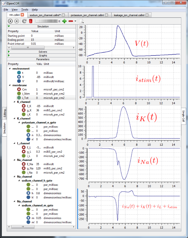
Fig. 29 Results from OpenCOR for the Hodgkin Huxley (HH) CellML model. The top panel shows the generated action potential. Note that the stimulus current is not really needed as the background outward leakage current is enough to drive the membrane potential up to the threshold for sodium channel opening.
Important note
It is often convenient to have the sub-models – in this case the sodium_ion_channel.cellml model, the potassium_ion_channel.cellml model and the leakage_ion_channel.cellml model - loaded into OpenCOR at the same time as the high level model (HH.cellml), as shown in Fig. 30 . If you make changes to a model in the CellML Text view, you must save the file (CTRL-S) before running a new simulation since the simulator works with the saved model. Furthermore, a change to a sub-model will only affect the high level model which imports it if you also save the high level model (or use the Reload option under the File menu). An asterisk appears next to the name of a file when a change has been made and the file has not been saved. The asterisk disappears when the file is saved.

Fig. 30 The HH.cellml model and its three sub-models are available under separate tabs in OpenCOR.
Footnotes