A model of ion channel gating and current: Introducing CellML units
A good example of a model based on a first order equation is the one used by Hodgkin and Huxley [AAF52] to describe the gating behaviour of an ion channel (see also next three sections). Before we describe the gating behaviour of an ion channel, however, we need to explain the concepts of the ‘Nernst potential’ and channel conductance.
An ion channel is a protein or protein complex embedded in the bilipid membrane surrounding a cell and containing a pore through which an ion \(Y^{+}\) (or \(Y^{-}\)) can pass when the channel is open. If the concentration of this ion is \(\left\lbrack Y^{+} \right\rbrack_{o}\) outside the cell and \(\left\lbrack Y^{+} \right\rbrack_{i}\) inside the cell, the force driving an ion through the pore is calculated from the change in entropy.
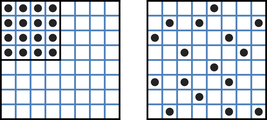
Fig. 12 Distribution of microstates in a system [J97]. The 16 particles in a confined region (left) have only one possible arrangement (W = 1) and therefore zero entropy (\(k_{B}\text{lnW}=0\)). When the barrier is removed and the number of possible locations for each particle increases 4x (right), the number of possible arrangements for the 16 particles increases by 416 and the increase in entropy is therefore \(ln(416)\) or \(16ln4\). The thermal energy (temperature) of the previously confined particles on the left has been redistributed in space to achieve a more probable (higher entropy) state. If we now added more particles to the container on the right, the concentration would increase and the entropy would decrease.
Entropy \(S\) (\(J.K^{-1}\)) is a measure of the number of microstates available to a system, as defined by Boltzmann’s equation \(S = k_{B}\text{lnW}\), where \(W\) is the number of ways of arranging a given distribution of microstates of a system and \(k_{B}\) is Boltzmann’s constant[1]. The driving force for ion movement is the dispersal of energy into a more probable distribution (see Fig. 12; cf. the second law of thermodynamics[2]).
The energy change \(\Delta q\) associated with this change of entropy \(\Delta S\) at temperature \(T\) is \(\Delta q = T\Delta S\) (J).
For a given volume of fluid the number of microstates \(W\) available to a solute (and hence the entropy of the solute) at a high concentration is less than that for a low concentration[3]. The energy difference driving ion movement from a high ion concentration \(\left\lbrack Y^{+} \right\rbrack_{i}\) (lower entropy) to a lower ion concentration \(\left\lbrack Y^{+} \right\rbrack_{o}\) (higher entropy) is therefore
\(\Delta q = T\Delta S = k_{B}T\left( \ln{\left\lbrack Y^{+} \right\rbrack_{o} - \ln\left\lbrack Y^{+} \right\rbrack_{i}} \right) = k_{B}T\ln\frac{\left\lbrack Y^{+} \right\rbrack_{o}}{\left\lbrack Y^{+} \right\rbrack_{i}}\) (\(J.ion^{-1}\))
or
\(\Delta Q = RT\ln\frac{\left\lbrack Y^{+} \right\rbrack_{o}}{\left\lbrack Y^{+} \right\rbrack_{i}}\) (\(J.mol^{-1}\)).
\(R = k_{B}N_{A} \approx 1.34x10^{-23} (J.K^{-1}) \text{x} 6.02x10^{23} (mol^{-1}) \approx 8.4 (J.mol^{-1}K^{-1})\) is the ‘universal gas constant’[4]. At 25°C (298K), \(\text{RT} \approx 2.5 kJ.mol^{-1}\).
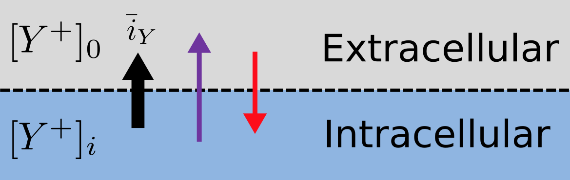
Fig. 13 The balance between entropic and electrostatic forces determines the Nernst potential.
Every positively charged ion that crosses the membrane raises the potential difference and produces an electrostatic driving force that opposes the entropic force (see Fig. 13). To move an electron of charge e (\(\approx 1.6x10^{-19}\) C) through a voltage change of \(\Delta\phi\) (V) requires energy \(e\Delta\phi\) (J) and therefore the energy needed to move an ion \(Y^{+}\) of valence z=1 (the number of charges per ion) through a voltage change of \(\Delta\phi\) is \(\text{ze}\Delta\phi\) (\(J.ion^{-1}\)) or \(\text{ze}N_{A}\Delta\phi\) (\(J.mol^{-1}\)). Using Faraday’s constant \(F = eN_{A}\), where \(F \approx 0.96x10^{5} C.mol^{-1}\), the change in energy density at the macroscopic scale is \(\text{zF}\Delta\phi\) (\(J.mol^{-1}\)).
No further movement of ions takes place when the force for entropy driven ion movement exactly equals the opposing electrostatic driving force associated with charge movement:
\(\text{zF}\Delta\phi = \text{RT}\ln\frac{\left\lbrack Y^{+} \right\rbrack_{o}}{\left\lbrack Y^{+} \right\rbrack_{i}}\) (\(J.mol^{-1}\)) or \(\Delta\phi = E_{Y} = \frac{\text{RT}}{\text{zF}}\ln\frac{\left\lbrack Y^{+} \right\rbrack_{o}}{\left\lbrack Y^{+} \right\rbrack_{i}}\) (\(J.C^{-1}\) or V)
where \(E_{Y}\) is the ‘equilibrium’ or ‘Nernst’ potential for \(Y^{+}\). At 25°C (298K), \(\frac{\text{RT}}{F} = \frac{2.5x10^{3}\ }{0.96x10^{5}} (J.C^{-1}) \approx 25mV\).
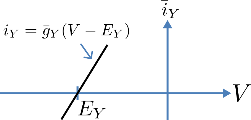
Fig. 14 Open channel linear current-voltage relation
For an open channel the electrochemical current flow is driven by the open channel conductance \({\overset{\overline{}}{g}}_{Y}\) times the difference between the transmembrane voltage \(V\) and the Nernst potential for that ion:
\({\overset{\overline{}}{i}}_{Y}\mathbf{=}{\overset{\overline{}}{g}}_{Y}\left( V - E_{Y} \right)\).
This defines a linear current-voltage relation (‘Ohms law’) as shown in Fig. 14. The gates to be discussed below modify this open channel conductance.
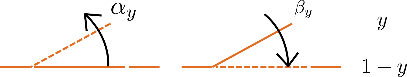
Fig. 15 Ion channel gating kinetics. y is the fraction of gates in the open state. α_y and β_y are the rate constants for opening and closing, respectively.
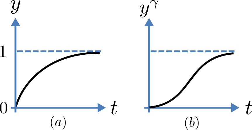
Fig. 16 Transient behaviour for one gate (left) and γ gates in series (right). Note that the right hand graph has an initial S-shaped increase, reflecting the multiple gates in series.
To describe the time dependent transition between the closed and open states of the channel, Hodgkin and Huxley introduced the idea of channel gates that control the passage of ions through a membrane ion channel. If the fraction of gates that are open is y, the fraction of gates that are closed is \(1-y\), and a first order ODE can be used to describe the transition between the two states (see Fig. 15):
\(\frac{\text{dy}}{\text{dt}} = \alpha_{y}\left( 1 - y \right) - \beta_{y}\text{.y}\)
where \(\alpha_{y}\)is the opening rate and \(\beta_{y}\) is the closing rate.
The solution to this ODE is
\(y = \frac{\alpha_{y}}{\alpha_{y} + \beta_{y}} + Ae^{- \left( \alpha_{y} + \beta_{y} \right)t}\)
The constant \(A\) can be interpreted as \(A = y\left( 0 \right) - \frac{\alpha_{y}}{\alpha_{y} + \beta_{y}}\) as in the previous example and, with \(y\left( 0 \right) = 0\) (i.e. all gates initially shut), the solution looks like Fig. 16(a).
The experimental data obtained by Hodgkin and Huxley for the squid axon, however, indicated that the initial current flow began more slowly (Fig. 16(b)) and they modelled this by assuming that the ion channel had \(\gamma\) gates in series so that conduction would only occur when all gates were at least partially open. Since \(y\) is the probability of a gate being open, \(y^{\gamma}\) is the probability of all \(\gamma\) gates being open (since they are assumed to be independent) and the current through the channel is
\(i_{Y} = {\overset{\overline{}}{i}}_{Y}y^{\gamma} = y^{\gamma}{\overset{\overline{}}{g}}_{Y}\left( V - E_{Y} \right)\)
where \({\overset{\overline{}}{i}}_{Y}{= \overset{\overline{}}{g}}_{Y}\left( V - E_{Y} \right)\) is the steady state current through the open gate.
We can represent this in OpenCOR with a simple extension of the first order ODE model, but in developing this model we will also demonstrate the way in which CellML deals with units.
Note that the decision to deal with units in CellML, rather than just ignoring them or insisting that all equations are represented in dimensionless form, was made in order to be able to check the physical consistency of all terms in each equation[5].
There are seven base physical quantities defined by the International d’Unités (SI)[6]. These are (with their SI units):
length (meter or m)
time (second or s)
amount of substance (mole)
temperature (K)
mass (kilogram or kg)
current (amp or A)
luminous intensity (candela).
All other units are derived from these seven. Additional derived units that CellML defines intrinsically (with their dependence on previously defined units) are: Hz (\(s^{-1}\)); Newton, N (\(kg.m.s^{-1}\)); Joule, J (\(N.m\)); Pascal, Pa (\(N.m^{-2}\)); Watt, W (\(J.s^{-1}\)); Volt, V (\(W.A^{-1}\)); Siemen, S (\(A.V^{-1}\)); Ohm, \(\Omega\) (\(V.A^{-1}\)); Coulomb, C (\(s.A\)); Farad, F (\(C.V^{-1}\)); Weber, Wb (\(V.s\)); and Henry, H (\(Wb.A^{-1}\)). Multiples and fractions of these are defined as follows:
Prefix |
deca |
hecto |
kilo |
mega |
giga |
tera |
peta |
exa |
zetta |
yotta |
||
Multiples |
Symbol |
da |
h |
k |
M |
G |
T |
P |
E |
Z |
Y |
|
Factor |
\(10^0\) |
\(10^{1}\) |
\(10^{2}\) |
\(10^{3}\) |
\(10^{6}\) |
\(10^{9}\) |
\(10^{12}\) |
\(10^{15}\) |
\(10^{18}\) |
\(10^{21}\) |
\(10^{24}\) |
|
Prefix |
deci |
centi |
milli |
micro |
nano |
pico |
femto |
atto |
zepto |
yocto |
||
Fractions |
Symbol |
d |
c |
m |
μ |
n |
p |
f |
a |
z |
y |
|
Factor |
\(10^{0}\) |
\(10^{-1}\) |
\(10^{-2}\) |
\(10^{-3}\) |
\(10^{-6}\) |
\(10^{-9}\) |
\(10^{-12}\) |
\(10^{-15}\) |
\(10^{-18}\) |
\(10^{-21}\) |
\(10^{-24}\) |
Units for this model, with multiples and fractions, are illustrated in the following CellML Text code[7]:
 1def model first_order_model as
 2    def unit millisec as
 3        unit second {pref: milli};
 4    enddef;
 5    def unit per_millisec as
 6        unit second {pref: milli, expo: -1};
 7     enddef;
 8    def unit millivolt as
 9        unit volt {pref: milli};
10    enddef;
11    def unit microA_per_cm2 as
12        unit ampere {pref: micro};
13        unit metre {pref: centi, expo: -2};
14    enddef;
15    def unit milliS_per_cm2 as
16        unit siemens {pref: milli};
17        unit metre {pref: centi, expo: -2};
18    enddef;
19    def comp ion_channel as
20        var V: millivolt {init: 0};
21        var t: millisec {init: 0};
22        var y: dimensionless {init: 0};
23        var E_y: millivolt {init: -85};
24        var i_y: microA_per_cm2;
25        var g_y: milliS_per_cm2 {init: 36};
26        var gamma: dimensionless {init: 4};
27        var alpha_y: per_millisec {init: 1};
28        var beta_y: per_millisec {init: 2};
29        ode(y, t) = alpha_y*(1{dimensionless}-y)-beta_y*y;
30        i_y = g_y*pow(y, gamma)*(V-E_y);
31     enddef;
32enddef;
The solution of these equations for the parameters indicated above is illustrated in Fig. 17.
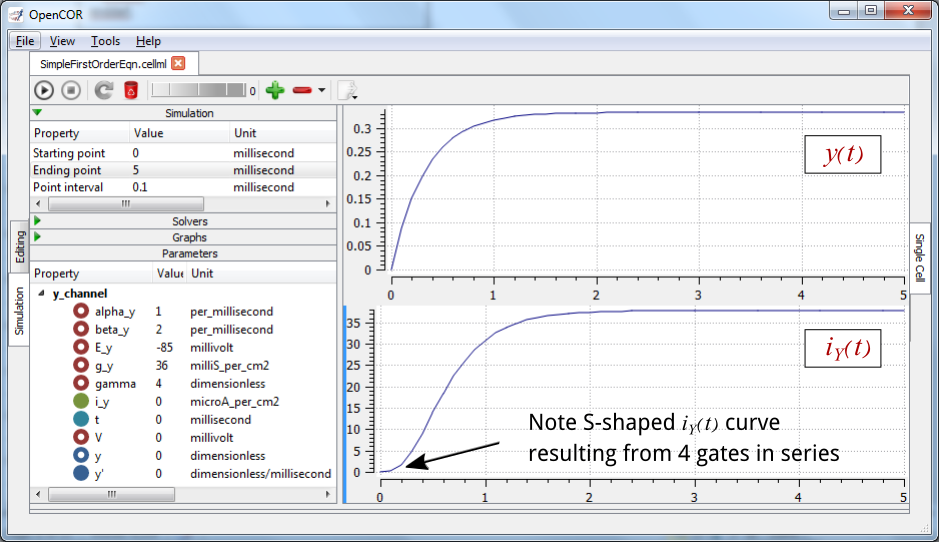
Fig. 17 The behaviour of an ion channel with \(\gamma = 4\) gates transitioning from the closed to the open state at a membrane voltage \(V = 0\) (OpenCOR link). The opening and closing rate constants are \(\alpha_{y} = 1\) ms-1 and \(\beta_{y} = 2\) ms-1. The ion channel has an open conductance of \({\overset{\overline{}}{g}}_{Y} = 36\) mS.cm-2 and an equilibrium potential of \(E_{Y} = - 85\) mV. The upper transient is the response \(y\left( t \right)\) for each gate and the lower trace is the current through the channel. Note the slow start to the current trace in comparison with the single gate transient \(y\left( t \right)\).
The model of a gated ion channel presented here is used in the next two sections for the neural potassium and sodium channels and then in Section 11 for cardiac ion channels. The gates make the channel conductance time dependent and, as we will see in the next section, the experimentally observed voltage dependence of the gating rate constants \(\alpha_{y}\) and \(\beta_{y}\) means that the channel conductance (including the open channel conductance) is voltage dependent. For a partially open channel (\(y < 1\)), the steady state conductance is \(\left( y_{\infty} \right)^{\gamma}{.\overset{\overline{}}{g}}_{Y}\), where \(y_{\infty} = \frac{\alpha_{y}}{\alpha_{y} + \beta_{y}}\). Moreover the gating time constants \(\tau = \frac{1}{\alpha_{y} + \beta_{y}}\) are therefore also voltage dependent. Both of these voltage dependent factors of ion channel gating are important in explaining channel properties, as we show now for the neural potassium and sodium ion channels.
Footnotes