A simple first order ODE
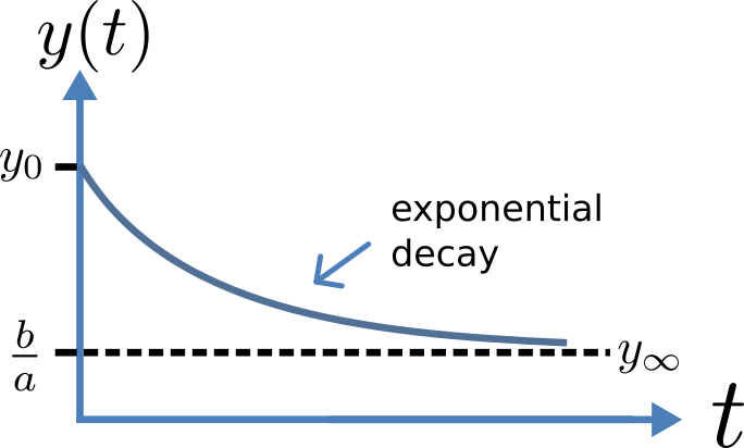
Fig. 6 Solution of 1st order equation.
The simplest example of a first order ODE is
with the solution
where \(y\left( 0 \right)\) or \(y_{0}\), the value of \(y\left( t \right)\) at \(t = 0\), is the initial condition. The final steady state solution as \(t \rightarrow \infty\) is \(y\left( \left. \ t \right|_{\infty} \right) = y_{\infty} = \frac{b}{a}\) (see Figure 6). Note that \(t = \tau = \frac{1}{a}\) is called the time constant of the exponential decay, and that
At \(t = \tau\) , \(y\left( t \right)\) has therefore fallen to \(\frac{1}{e}\) (or about 37%) of the difference between the initial (\(y\left( 0 \right)\)) and final steady state ( \(y\left( \infty \right)\)) values[1].
Choosing parameters \(a = \tau = 1;b = 2\) and \(y\left( 0 \right) = 5\), the CellML Text for this model is
def model first_order_model as
    def comp main as
        var t: dimensionless {init: 0};
        var y: dimensionless {init: 5};
        var a: dimensionless {init: 1};
        var b: dimensionless {init: 2};
        ode(y,t)=-a*y+b;
    enddef;
enddef;
The solution by OpenCOR is shown in Fig. 7(a) for these parameters (a decaying exponential) and in Fig. 7(b) for parameters \(a = 1;b = 5\) and \(y\left( 0 \right) = 2\) (an inverted decaying exponential). Note the simulation panel with Ending point=10, Point interval=0.1. Try putting \(a = - 1\).
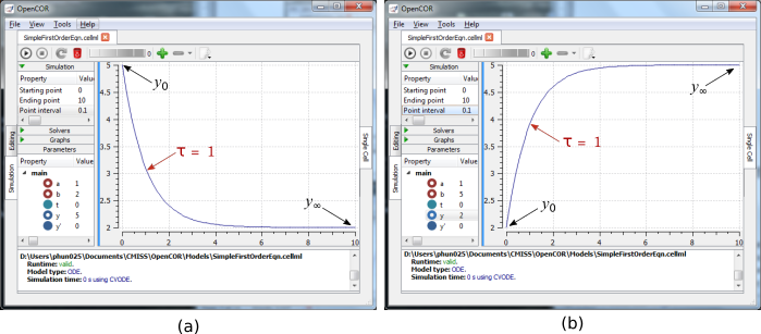
Fig. 7 OpenCOR output \(y\left( t \right)\) for the simple ODE model with parameters (a) \(a = 1;b = 2\) and \(y\left( 0 \right) = 5\) (OpenCOR link), and (b) \(a = 1;b = 5\) and \(y\left( 0 \right) = 2\). The red arrow indicates the point at which the trace reaches the time constant \(\tau\) (\(e^{- 1}\) or \(\approx 37\%\) of the difference between the initial and final solution values). The black arrows indicate the initial and final (steady state) solutions. Note that the parameters on the left have been reset to their initial values for this figure - normally they would be at their final solution values.
These two solutions have the same exponential time constant (\(\tau = \frac{1}{a} = 1\)) but different initial and final (steady state) values.
The exponential decay curve shown on the left in Fig. 7 is a common feature of many models and in the case of radioactive decay (for example) is a statement that the rate of decay (\(- \frac{\text{dy}}{\text{dt}}\)) is proportional to the current amount of substance (\(y\)). This is illustrated on the NZ$100 note (should you be lucky enough to possess one), shown in Figure 8.
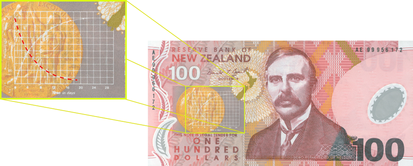
Fig. 8 The exponential curve representing the naturally occurring radioactive decay explained by the New Zealand Noble laureate Sir Ernest Rutherford - best known for ‘splitting the atom’. This may be the only bank note depicting the mathematical solution of a first order ODE.
Footnotes